Calibration

Flydra calibration data (also, in the flydra source code, a reconstructor) consists of:

• parameters for a linear pinhole camera model (including intrinsic and extrinsic calibration).
• parameters for non-linear distortion.
• (optional) a scale factor and units (e.g. 1000.0 and millimeters). If not specified these default to 1.0 and meters. If these are specified they specify how to convert the native units into meters (the scale factor) and the name of the present units. (Meters are the units used the dyanmic models, and otherwise have no significance.)

See Calibration files and directories - overview for a discussion of the calibration file formats.

Generating a calibration using MultiCamSelfCal

The basic idea is that you will save raw 2D data points which are easy to track and associate with a 3D object. Typically this is done by waving an LED around.

For this to work, the 2D/3D data association problem must be trivial. Only a single 3D point should be generating 2D points, and every 2D point should come from the (only) 3D point. (Missing 2D points are OK; occlusions per se do not cause problems, whereas insufficient or false data associations do.)

(3D trajectories, which can only come from having a calibration and solving the data association problem, will not be used for this step, even if available. If a calibration has already been used to generate Kalman state estimates, the results of this data association will be ignored.)

Typically, about 500 points distributed throughout the tracking volume will be needed for the MATLAB MultiCamSelfCal toolbox to complete successfully. Usually, however, this will mean that you save many more points and then sub-sample them later. See the config.cal.USE_NTH_FRAME parameter below.

Saving the calibration data in flydra_mainbrain

Start saving data normally within the flydra_mainbrain application. Remember that only time points with more than 2 cameras returning data will be useful, and that time points with more than 1 detected view per camera are useless.

Walk to the arena and wave the LED around. Make sure it covers the entire tracking volume, and if possible, outside the tracking volume, too.

Exporting the data for MultiCamSelfCal

Now, you have saved an .h5 file. To export the data from it for calibration, run:

flydra_analysis_generate_recalibration --2d-data DATAFILE2D.h5 \
  --disable-kalman-objs DATAFILE2D.h5

You should now have a new directory named DATAFILE2D.h5.recal. This contains the raw calibration data (synchronized 2D points for each camera) in a format that the MATLAB MultiCamSelfCal can understand, the calibration directory.

Running MultiCamSelfCal

NOTE: This section is out of date. The new version of MultiCamSelfCal does not require MATLAB and can be run purely with Octave. The new version of MultiCamSelfCal is available from https://github.com/strawlab/MultiCamSelfCal

Edit the file kookaburra/MultiCamSelfCal/CommonCfgAndIO/configdata.m.

In the SETUP_NAME section, there a few variables you probably want to examine:

• In particular, set config.paths.data to the directory where your calibration data is. This is the output of the flydra_analysis_generate_recalibration command. Note: this must end in a slash (/).
• config.cal.GLOBAL_ITER_THR is the criterion threshold reprojection error that all cameras must meet before terminating the global iteration loop. Something like 0.8 will be decent for an initial calibration (tracking an LED), but tracking tiny Drosophila should enable you to go to 0.3 or so (in other words, generating calibration data with the Running MultiCamSelfCal method). To estimate the non-linear distortion (often not necessary), set this small enough that gocal runs non-linear parameter estimation at least once. This non-linear estimation step fits the radial distortion term.
• config.cal.USE_NTH_FRAME if your calibration data set is too massive, reduce it with this variable. Typically, a successful calibration will have about 300-500 points being used in the final calibration. The number of points used will be displayed during the calibration step (For example, “437 points/frames have survived validations so far”.)
• config.files.idxcams should be set to [1:X] where X is the number of cameras you are using.
• config.cal.UNDO_RADIAL should be set to 1 if you are providing a .rad file with non-linear distortion parameters.

The other files to consider are MultiCamSelfCal/CommonCfgAndIO/expname.m and kookaburra/MultiCamSelfCal/MultiCamSelfCal/BlueCLocal/SETUP_NAME.m. The first file returns a string that specifies the setup name, and consequently the filename (written above as SETUP_NAME) for the second file. This second file contains (approximate) camera positions which are used to determine the rotation, translation, and scale factors for the final camera calibration. The current dynamic models operate in meters, while the flydra code automatically multiplies post-calibration 3D coordinates by 1000 (thus, converting millimeters to meters) unless a file named calibration_units.txt specifies the units. Thus, unless you create this file, use millimeters for your calibration units.

Run MATLAB (e.g. matlab -nodesktop -nojvm). From the MATLAB prompt:

cd kookaburra/MultiCamSelfCal/MultiCamSelfCal/
gocal

When the initial mean reprojection errors are displayed, numbers of 10 pixels or less bode pretty well for this calibration to converge. It is rare, to get a good calibration when the first iteration has large reprojection errors. Running on a fast computer (e.g. Core 2 Duo 2 GHz), a calibration shouldn’t take more than 5 minutes before looking pretty good if things are going well. Note that, for the first calibration, it may not be particularly important to get a great calibration because it will be redone due to the considerations listed in Running MultiCamSelfCal.

Advanced: automatic homography (alignment) using approximate camera positions

Let’s say your calibration had three cameras and you know their approximate positions in world coordinates. You can automatically compute the homography (rotate, scale, and translate) between your original calibration and the new calibration such that the calibrated camera positions will be maximally similar to the given approximate positions.

Create a file called, e.g. align-cams.txt. Each line contains the 3D coordinates of each camera. The order of the cameras must be the same as in the calibration. Now, simply run:

``flydra_analysis_align_calibration --orig-reconstructor cal20110309a2.xml --align-cams align-cams.txt --output-xml``

The aligned calibration will be in ORIGINAL_RECONSTRUCTOR.aligned.xml.

Advanced: using 3D trajectories to re-calibrate using MultiCamSelfCal

Often, it is possible (and desirable) to make a higher precision trajectory than that possible by waving an LED. For example, flying Drosophila are smaller and therefore more precisely localized points than an LED. Also, in setups in which cameras film through movable transparent material, flies fly in the final experimental configuration, which may have slightly different optics that should be part of your final calibration.

By default, you enter previously-tracked trajectory ID numbers and the 2D data that comprised these trajectories are output.

This method also saves a directory with the raw data expected by the Multi Camera Self Calibration Toolbox.

# NOTE: if your 2D and 3D data are in one file,
# don't use the "--2d-data" argument.
flydra_analysis_generate_recalibration DATAFILE3D.h5 EFILE \
   --2d-data DATAFILE2D.h5
# This will output a new calibration directory in
# DATAFILE3D.h5.recal

The EFILE above should have the following format (for example):

# These are the obj_ids of traces to use.
long_ids = [655, 646, 530, 714, 619, 288, 576, 645]
# These are the obj_ids of traces not to use (exluded
# from the list in long_ids)
bad=[]

Finally, run the Multi Cam Self Calibration procedure on the new calibration directory. Lower your threshold to, e.g., config.cal.GLOBAL_ITER_THR = .4;. You might want to adjust config.cal.USE_NTH_FRAME again to get the right number of data points. This is a precise calibration, it might take as many as 30 iterations and 15 minutes.

Aligning a calibration

Often, even if a calibration from MultiCamSelfCal creates reprojections with minimal error and the relative camera positions look OK, reconstructed world coordinates do not correspond with desired world coordinates. To align the calibration the flydra_analysis_calibration_align_gui program may be used:

flydra_analysis_calibration_align_gui DATAFILE3D.h5 --stim-xml=STIMULUS.xml

This results in a GUI that looks a bit like

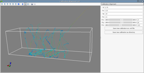
Using the controls on the right, align your data such that it corresponds with the 3D model loaded by STIMULUS.xml. When you are satisfied, click either of the save buttons to save your newly-aligned calibration.

Manually generating 3D points from images to use for alignment

You may want to precisely align some known 3D points. In this case the procedure is:

1. Use flydra_analysis_plot_kalman_2d to save a points.h5 file with the 3D positions resulting from the original calibration. In particular, use the hotkeys as defined in on_key_press().
2. Load points.h5 and a STIMULUS.xml file into flydra_analysis_calibration_align_gui and adjust the homography parameters until the 3D locations are correct.

Estimating non-linear distortion parameters

The goal of estimating non-linear distortions is to find the image warping such that images of real straight lines are straight in the images. There are two supported ways of estimating non-linear distortion parameters.:

1. Using the pinpoint GUI to manually adjust the warping parameters.
2. Using flydra_checkerboard to automatically estimate the parameters.

Use of flydra_checkerboard

flydra_checkerboard is a command-line program that generates a .rad file suitable for use by MultiCamSelfCal and the flydra tools (when included in a calibration directory).

The program is run with the name of a config file and possibly some optional command-line arguments.

If everything goes well, it will:

1. Detect the checkerboard corners
2. Cluster these corners into nearly orthogonal multi-segment pieces.
3. Estimate the best non-linear distortion that fits this multi-segments paths as closely as possible to straight lines.

The most important aspect of automatic corner detection is that long, multi-segment paths are detected near the edges of the image.

A minimal, but often sufficient, config file is given here. In this case, this file is named distorted2.cfg:

fname='distorted2.fmf' # The name of an .fmf movie with frames of a checkerboard
frames= 0,1,2,3 # The frames to extract checkerboard corners from
rad_fname = 'distorted2.rad' # The filename to save the results in.

A variety of other options exist:

use = 'raw' # The image pre-processing algorithm to use before
            # extracting checkerboard corners. In order of preference, the options are:
            # 'raw'       - the raw image, exactly as-is
            # 'rawbinary' - a thresholded image
            # 'binary'    - a background-subtracted and thresholded image
            # 'no_bg'     - a background-subtracted image
angle_precision_degrees=10.0 # Threshold angular difference between adjacent edges.
aspect_ratio = 1.0           # Aspect ratio of pixel spacing (1.0 is normal,
                                                              0.5 is vertically downsampled)

show_lines = False
return_early = False
debug_line_finding = False
epsfcn = 1e09
print_debug_info = False
save_debug_images = False

ftol=0.001
xtol=0
do_plot = False

K13 = 320 # center guess X
K23 = 240 # center guess Y

kc1 = 0.0 # initial guess of radial distortion
kc2 = 0.0 # initial guess of radial distortion

After adjusting these parameters, call flydra_checkerboard.

Critical to flydra_checkerboard is the ability to extract numerous checkerboard corners with few false positives. To ensure that this is happens, here are a few command line options that help debug the process:

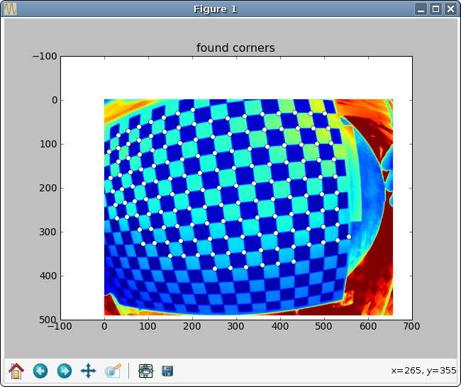
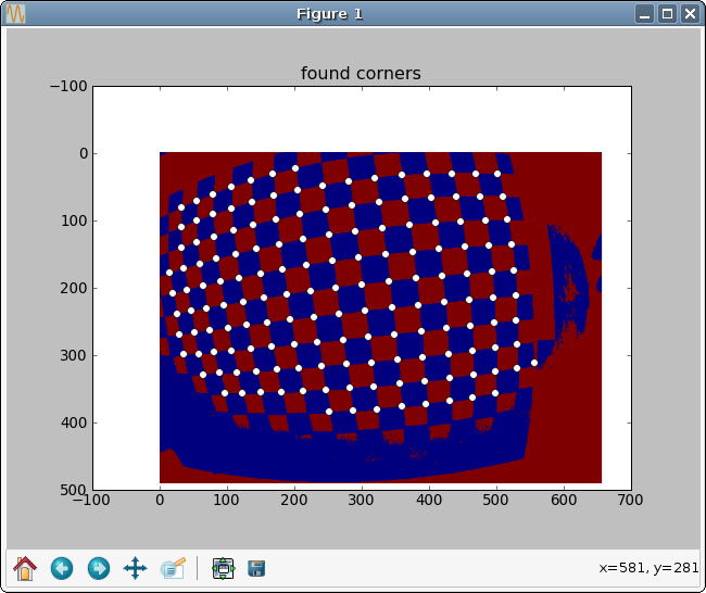
flydra_checkerboard distorted2.cfg --show-chessboard-finder-preview

The first image is a screenshot of the –show-chessboard-finder-preview output when using the ‘raw’ image. The detection of corners is good throughout most of the image, but lacking particularly in the lower left corner. The second image used the ‘rawbinary’ preprocessing mode. It appears to have detected more points, which is good.

Finding the horizontal and vertical edges

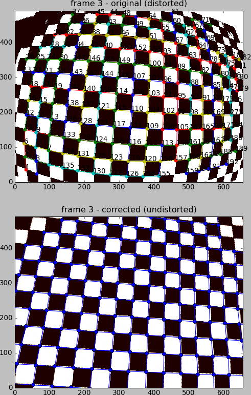
The next step is for flydra_checkerboard to find the grid of the chessboard. Run the folllowing command to see how well it does:

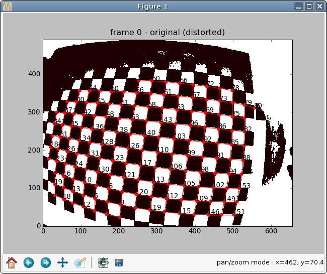
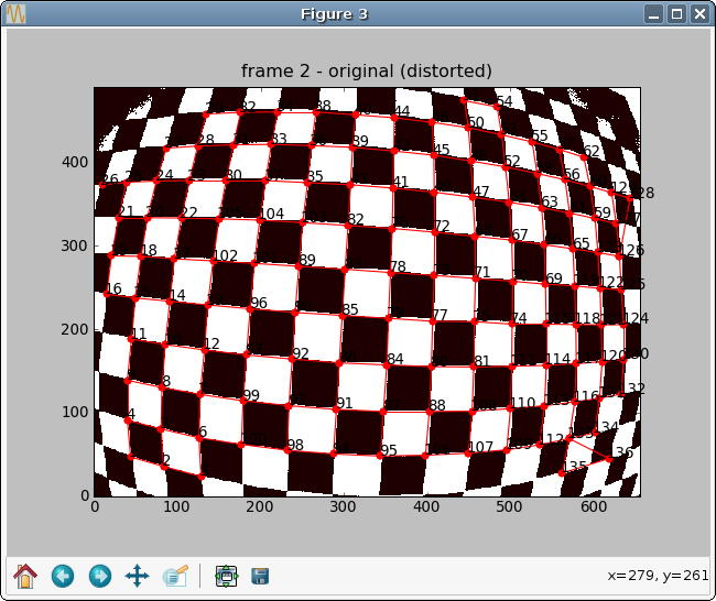
flydra_checkerboard distorted2.cfg --find-and-show1

Here are two sample images this was performed on. In the first image, we can see that the grid detection was very good, with no obvious mistakes. In the second example, the grid detection had a couple mistakes – one in the lower right corner and one in the upper right corner.

If everything looks good to this point, you may be interested in a final check with the –find-and-show2, which identifies individual paths. It is these paths that will be attempted to straighted in the optimization procedure to follow.

To actually estimate the radial distortion, call the command with no options:

flydra_checkerboard distorted2.cfg

This will begin a gradient descent type optimization and will hopefully return a set of good values. Note that you can seed the starting values for the parameters with the K13, K23, kc1, and kc2 parameters described above. Over time you should see the error decreasing, rapidly at first, and then more slowly.

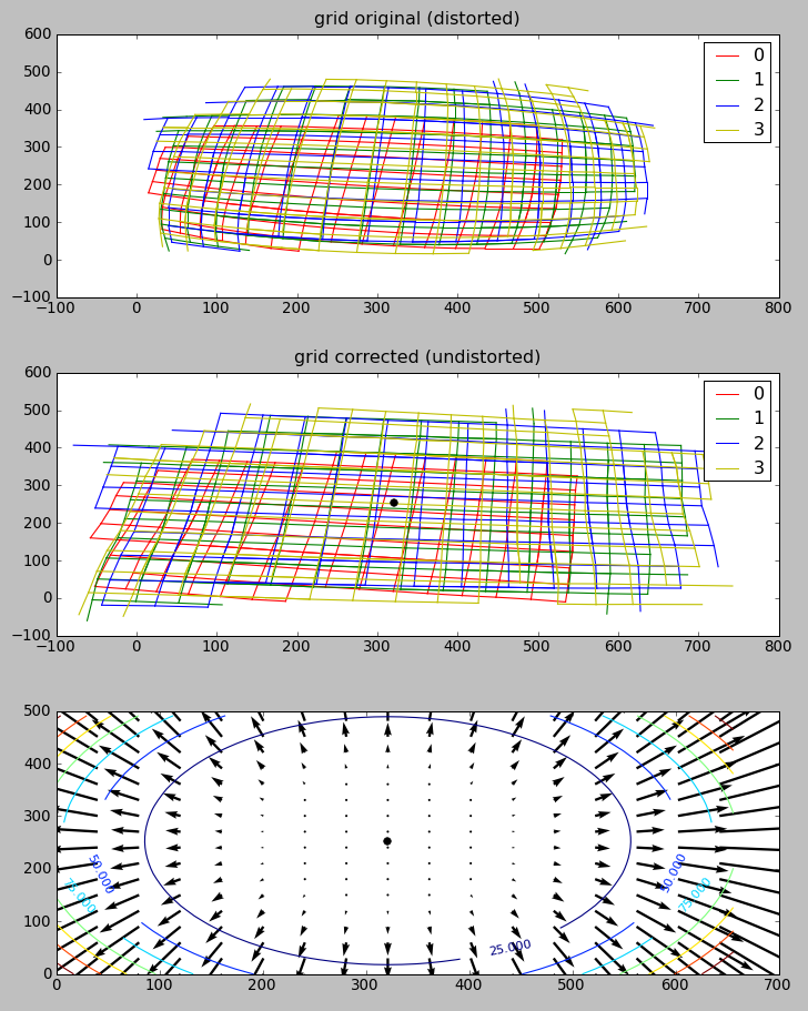
Once the optimization is done, you may visualize the results. This command reads the non-linear distortion terms from the .rad files:

flydra_checkerboard distorted2.cfg  --view-results

This command reads all the files, re-finds the corners, and plots several summary plots. The most importart thing is that straight lines look straight. In the example images below, the distortion estimation appears to have done a reasonably good job – the undistorted image has rather straight lines, and the “grid corrected” panel appears to show mostly straight (although not perfect) checkerboards.