old Trac wiki page about Flydra
This page was copied from the old Trac wiki page about Flydra and may have suffered some conversion issues.
Flydra is heavily based on the motmot packages.
See Andrew’s manuscript about flydra. Please send him any comments/questions/feedback about the manuscript as he is planning on submitting it.
Subpages about flydra
Scripts of great interest
- source(command: kdviewer, file: flydra/a2/kdviewer.py) 3D viewer of Kalmanized trajectories saved in .h5 data file. (This is newer version of source(file: flydra/analysis/flydra_analysis_plot_kalman_data.py) that uses TVTK.)
- source(command: flydra_kalmanize, file: flydra/kalman/kalmanize.py) re-analyze 2D data saved in .h5 data file using same Kalman filtering code as realtime analysis. Note: this will only run the causal Kalman filter, which allows re-segmenting the data into trajectories. However, another step, of running the non-causal smoothing algorithm, is typically desired. (See below for reasons why you might want to do this.)
- source(command: flydra_analysis_generate_recalibration, file: flydra/analysis/flydra_analysis_generate_recalibration.py) save 2D data from a previously saved .h5 file to perform a (re-)calibration. This new calibration typically has very low reprojection errors. Performing this step can use either 3D trajectories in the .h5 file in order to solve the correspondence problem (which 2D points from which cameras correspond to the same 3D point). Alternatively, if only (at most) a single point is tracked per camera per time point, they are assumed to be from the same 3D point. In this case, specify a start and stop frame.
ffpmegfor exampleffmpeg -b 2008000 -f mpeg2video -r 25 -i image%05d.png movie.mpeg- source(command: flydra_analysis_convert_to_mat, file: flydra/analysis/flydra_analysis_convert_to_mat.py) convert .h5 3D data to .mat for MATLAB; includes raw observations and realtime kalman filtered observations.
- source(command: data2smoothed, file: flydra/a2/data2smoothed.py) convert .h5 3D data to .mat file for MATLAB; returns only results of 2nd pass kalman smoothing and timestamps
- source(command: flydra_textlog2csv, file: flydra/a2/flydra_textlog2csv.py) save text log from .h5 file to CSV format (can be opened in Excel, for example)
Scripts of lesser interest
- source(command: flydra_analysis_filter_kalman_data.py, file: flydra/analysis/flydra_analysis_filter_kalman_data.py) export a subset of the Kalmanized trajectories in an .h5 file to a new (smaller) .h5 file.
- source(command: flydra_analysis_plot_kalman_2d.py, file: flydra/analysis/flydra_analysis_plot_kalman_2d.py) plot 2D data (x against y), including Kalmanized trajectories. (This is more-or-less the camera view.)
- source(command: plot_timeseries_2d_3d.py, file: flydra/a2/plot_timeseries_2d_3d.py plot_timeseries_2d_3d.py) plot 2D and 3D data against frame number. (This is a time series.)
- source(command: plot_timeseries.py, file: flydra/a2/plot_timeseries.py) plot 3D data against frame number. (This is a time series.)
- source(command: flydra_images_export, file: flydra/a2/flydra_images_export.py) export images from .h5 file.
Reasons to run flydra_kalmanize on your data, even though it’s already been Kalmanized
- Re-running uses all the 2D data, including that which was originally dropped during realtime transmission to the mainbrain.
- (If a time-budget for 3D calculations ever gets implemented, this running this will also bypass any time-budget based cuts.)
- You have a new (better) calibration.
- You have a new (better) set of Kalman parameters and model.
Image masking
Export camera views from the .h5 file:
flydra_images_export DATA20080402_115551.h5
This should have saved files named cam_id.bmp, (e.g. “cam1_0.bmp”). Open these in GIMP (the GNU image manipulation program).
Add an alpha channel: open the Layers dialog (if it’s not already open). Right click on the layer (called “Background”), then select “Add alpha channel”.
Convert to RGB: Use the “Image” menu in the menubar: “Image->Mode->RGB”. (It would be nice if flydra supported grayscale images in addition to RGB, but that’s not yet implemented.)
Use the free select tool (like a lasso), to select the region you want to ignore using the tool. Hints: You can select multiple areas by holding down the ‘shift’ key. You can drag the lasso outside of the image and it will just draw along the edge of the image. Next invert the selection “Select->Invert” and cut the region you want to track over (Ctrl-X).
The alpha channel may not have any values except 0 and 255, therefore if you are not completely sure, use LAYERS/TRANSPARENCY/THRESHOLD ALPHA in Gimp to create a clean alpha channel.
Here’s an example of what you’re looking for. The important point is that you’ll be tracking over the region where this image is transparent.
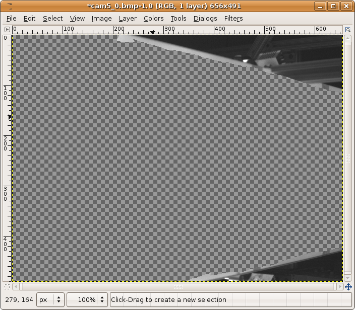
Finally, “File->Save As…” and save as a .png file. The default options are fine.
If you saved your file as “cam5_0_mask.png”, you would use this with a command like:
flydra_camera_node --mask-images=cam5_0_mask.png
in a launch file, this would for example look like this:
<node name="flydra_camera_node" pkg="ros_flydra" type="camnode" args="--num-buffers=100 --background-frame-alpha=0.01 --background-frame-interval=80 --num-points=6 --sleep-first=5 --mask-images=$(find flycave)/calibration/flycube1/oct_2013/Basler_21275576_mask.png:$(find flycave)/calibration/flycube1/oct_2013/Basler_21275577_mask.png:$(find flycave)/calibration/flycube1/oct_2013/Basler_21283674_mask.png:$(find flycave)/calibration/flycube1/oct_2013/Basler_21283677_mask.png:$(find flycave)/calibration/flycube1/oct_2013/Basler_21359437_mask.png" />
Watch out! The masks in the launch file (e.g. ‘flydra.node’ are in the OPPOSITE ORDER than the camera names in the .yaml file (e.g. ‘flydra.yaml’). You can check this in the console output of the camnode:
----------------------------------------------------------------------------------------------------
Camera guid ='Basler_21275577'
has mask image: '/opt/ros/ros-flycave.electric.boost1.46/flycave/calibration/flycube1/oct_2013/Basler_21275577_mask.png'
Note that, as flydra_camera_node supports multiple cameras, you may specify multiple mask images – one for each camera. In these case, they are separated by the (OS-specific) path separator. This is ‘:’ on linux.
Latency/performance of flydra
Back in March 2007 or so, Andrew Straw measured the total latency of flydra. At the time of writing (November 6, 2007) I remember the shorter latencies to be approx. 55 msec. Most latencies were in this range, but not being a hard-realtime system, some tended to be longer. Most latencies, however were under 80 msec.
Today (November 6, 2007) I have done some more experimentation and added some profiling options. Here’s the breakdown of times:
- 20 msec from the Basler A602f cameras. (This is a fundamental limit of 1394a, as it takes this long for the image to get to the host computer. 1394b or GigE cameras would help.)
- 10 msec for local, 2D image processing and coordinate extraction on a 3.0 GHz Pentium 4 (w/HT) computer when
flydra_camera_nodeis using--num-points=3.- 1 msec transmission delay to the Main Brain.
- 15-30 msec for 3D tracking when
flydra_camera_nodeis using--num-points=3. (This drops to less than 10 msec with--num-points=1.) This test was performed with an Intel Core 2 Duo 6300 @ 1.86GHz as the Main Brain.
The values above add up roughly to the values I remember from earlier in 2007, so I guess this is more-or-less what was happening back then.
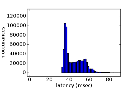
As of Nov. 16, 2007, the check_atmel script was used to generate
this figure, which is total latency to reconstructed 3D on the
mainbrain with flydra_camera_node using --num-points=2. This
includes the 20 msec Basler A602f latency, so presumably for GigE,
you’d subtract approx. 15 msec. Faster 2D camera computers would
probably knock off another 5 msec.
As of Feb. 20, 2008, the LED_test_latency script was used to test total latency from LED on to UDP packets with position information. This total latency was between 34-70 msec, with the 3D reconstruction latency being from about 25-45 msec. Note that these are from the initial onset of illumination, which may have different amounts of latencies than ongoing tracking.
Profiling
To profile the realtime Kalman filter code, first run the
flydra_mainbrain app with the --save-profiling-data
option. You will have to load the 3D calibration, synchronize the
cameras and begin tracking. The data sent to the Kalman tracker is
accummulated to RAM and saved to file when you quit the program. There
is no UI indication this is happening except when you finally quit it
will mention the filename. With the saved data file, run
source(command: kalman_profile.py, file: flydra/kalman/kalman_profile.py). This will generate profiling output that can be
opened in kcachegrind.
Flydra simulator
Option 1: Play FMFs through flydra_camera_node
This approach requires pre-recorded .fmf files.
Run the mainbrain:
REQUIRE_FLYDRA_TRIGGER=0 flydra_mainbrain
Now run an image server:
flydra_camera_node --emulation-image-sources full_20080626_210454_mama01_0.fmf --wx
Option 2: Play .h5 file
This approach is not yet implemented.